Discretizing Continuous SSMs

This post builds on my introduction to Mamba — if you haven’t read that yet, I’d recommend checking it out first for the full context on State Space Models.

As a quick refresher, SSMs are characterized by these continuous equations that map functions to functions. The continuous view gives us a function-to-function mapping, but in practice we’re working with discrete sequences of tokens, embeddings, or time steps — not continuous functions.

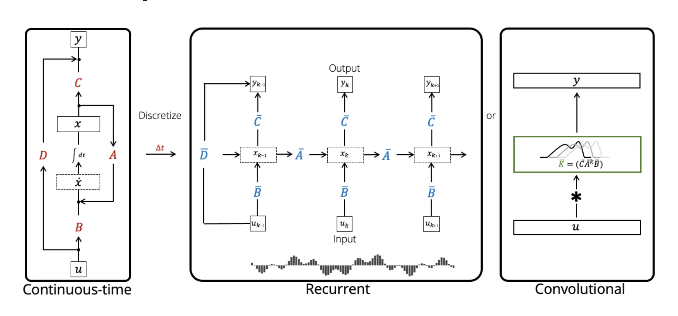
We need to discretize this to actually implement it on computers and train with gradient descent. Let’s dive into the math behind how this discretization actually works.

Proving the Discrete Form

Let’s start with the fundamental SSM equations in continuous form:

\[\begin{aligned} x'(t) &= Ax(t) + Bu(t) \\ y(t) &= Cx(t) + Du(t) \end{aligned}\]

These give us a function-to-function mapping \(u(t) \mapsto y(t)\) parameterized by \(A\), \(B\), \(C\), and \(D\) (fixed “latent” parameters), where \(x(t)\) is a latent representation satisfying the ODE.

The second equation \(y(t) = Cx(t) + Du(t)\) is just a linear transformation of our latent state \(x(t)\) plus a skip connection — \(D\) acts as a simple bias term that we can handle separately. The real challenge is discretizing the first equation, the ODE that governs how \(x(t)\) evolves. Let’s drop black-boxing things this time. How do we actually go from this continuous form to some discretization?

We can solve the top equation as below:

\[\begin{aligned} \frac{dx}{dt} &= Ax + Bu, \\ \frac{dx}{dt} - Ax &= Bu, \\ e^{-At} \left(\frac{dx}{dt} - Ax \right) &= e^{-At} Bu, \\ e^{-At} \frac{dx}{dt} - e^{-At}Ax &= e^{-At} Bu, \\ \frac{d}{dt}\left(e^{-At}x(t)\right) &= e^{-At} Bu, \\ x(t) &= e^{At}x_0 + e^{At} \int e^{-At} Bu(t) \, dt, \end{aligned}\]

So, between two states \(t_a\) and \(t_b\), we have

\[x(t_b) = e^{A(t_b - t_a)}(x_a + \int_{t_a}^{t_b} e^{-At} B_t u_t \, dt)\]

Heuristically, \(x_a\) is our initial state, \(B_t\) is the “control” we’re adding to the system over time, and \(u_t\) is our input. Discretizing the system, we then get

\[x_b = e^{A(\Delta_a + \dots + \Delta_{b-1})}(x_a + \sum_{i=a}^{b-1} e^{-A(\Delta_a + \dots + \Delta_i)} B_i u_i \Delta_i)\]

So, we can define a recurrent relationship to represent the evolution of terms over time in the format

\[x_i = p_A^i x_a + p_B^i\]

We get an initial pair \((p_A^a, p_B^a) = (e^{A\Delta_a}, B_a u_a \Delta_a)\) from our first discrete time point. From there, we have the recursive relationship

\[(p_A^i, p_B^i) = (e^{A\Delta_i}p_A^{i-1}, e^{A \Delta_i}p_B^{i-1} + B_i u_i \Delta_i)\]

so we can compute \(x_i = p_A^i x_0 + p_B^i\) pretty easily. The key insight is that if we can efficiently compute \(p_A^i\) and \(p_B^i\), then we can solve for any \(x_i\) quickly — which is exactly what the parallelization will give us.

Now, we have a concrete recursive relationship that — if you squint — looks like the recursive relationship we discussed regarding Linear RNNs in my original Mamba post. If you play around with the function, you’ll quickly realize that it’s associative:

\[f((p_A^1, p_B^1), (p_A^2, p_B^2)) = (p_A^1 p_A^2, p_A^1 p_B^1 + p_B^2)\]

which is basically the same associative function from Linear RNNs:

\[f((W_1, x_1), (W_2, x_2)) = (W_1 W_2, W_1 x_1 + x_2)\]

Thus, a modification of the Blelloch parallel prefix scan applies, and we can parallelize the computation in \(O(\log N)\) sequential steps. Once we have all the \(x_i\) states, computing the outputs \(y_i = Cx_i + Du_i\) is just a simple linear transformation and bias as we discussed earlier.

This is the core system that enables SSMs to work efficiently during inference. And luckily, because we have already computed all the \(p_A^i\), \(p_B^i\), and \(x_i\) values during the forward pass, we can cache them and use them during backpropagation!