Mamba: Selective State Space Modeling

This is a blog post regarding a talk I gave at K-Scale Labs to help everyone understand Mamba. The slides are here. State Space Models (SSMs) are one of the few machine learning archetypes that is competitive with Mamba in both inference speed and effectiveness — not to mention, they have some pretty cool intuition!

Papers + Resources

Some sources to look for more insight + math:

• The Original Mamba Paper
• DeepMind’s Linear RNN Paper
• State Space Models from HazyResearch
• HuggingFace SSM Introduction
• An Annotated SSM Implementation
• Mamba from Scratch by Algorithmic Simplicity

Introduction

What’s the problem with transformers?

There are a few:

• During qkv, calculating the attention score of each token (relative to every other) is $O(N^2)$ according to the length of the context window.
• Further, the quadratically-growing key-value cache needs to be stored alongside the model during inference.
• Moreover, having a context window at all is rather limiting

If we can address these problems with a different architecture, we can hopefully be better at long-range tasks, synthesizing speech and video (which are packed with context), training models quicker, and inference on smaller devices.

What are these “State Space Models (SSMs)”?

SSMs are characterized by two equations $\begin{aligned} x'(t) &= Ax(t) + Bu(t) \\ y(t) &= Cx(t) + Du(t) \end{aligned}$

However, we can simply interpret this as a function-to-function mapping $u(t) \mapsto y(t)$ parameterized by $A$, $B$, $C$, and $D$ (fixed “latent” parameters). Then, $x(t)$ is a latent representation satisfying the ODE. The important aspect of SSMs is that they have three views:

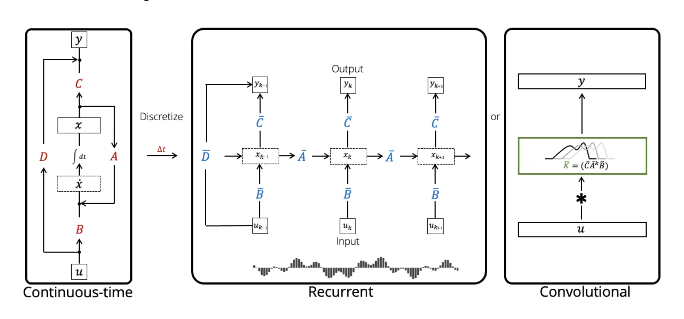
1. Continuous: This is simply our original equation — a function-to-function mapping of $u(t) \mapsto y(t)$ following the equation denoted above.
2. Recurrent: We can map our linear ODE to discrete steps in an RNN, with similar intuition for how we approach Flow Matching (see slide 4). We essentially turn our function-to-function mapping into a sequence-to-sequence mapping through interpolation

$\begin{aligned} x_k &= Ax_{k-1} + Bu_k \\ y_k &= Cx_k + Du_k \end{aligned}$

1. Convolutional: We unroll our recurrent view, solving $N$ steps ahead with the recurrence to get a kernel of size $N$, replugging-in values such that

$x_0 = \overline{B}u_0 \quad x_1 = \overline{A}B u_0 + \overline{B}u_1 \quad x_2 = \overline{A}^2 B u_0 + \overline{A}B u_1 + \overline{B}u_2 \quad \cdots$

Each of these views have tradeoffs, but the key version we want to focus on is the recurrent view. It has effectively no context window (unlike the convolutional view), which addresses the issue we have with transformers. On the other hand, it has a efficient constant time inference (unlike the continuous view), which once again addresses another problem we had with transformers.

However, recurrent networks are not easily parallelizable in training, as each inference is dependent on the previous time-step. Additionally, we’re at risk of vanishing/exploding gradients. How do we fix these problems?

Let’s drop the state space model idea — at this point, SSMs are an RNN that has its roots in continuous space and the possibility to become a convolution. Contrarily, an RNN models information statefully by being able to merge all of its previously seen context into one state.

Linear RNNs

Parallelizing

Having an activation function makes our calculations way too complicated and difficult to parallelize. What we really want is a way to calculate the accumulation of all an RNN’s layer multiplications quickly and easily. For each iteration with

$h_t = f_W(h_{t-1}, x_t)$

we can’t possibly expect condense these calculations quickly with a nonlinear activation function like $\tanh$ Instead, let’s remove the activation function so we’re left with

$f_W(h, x) = W_h h + W_x x$

How do we parallelize this? If we think about the Blelloch algorithm for parallel prefix sum, we can find some inspiration. With Blelloch, we are able to take the prefix sum of an array of length $n$ in $O(\log(N))$ sequential steps through parallelization simply because the addition property is associative. We do this by accumulating the sum over different step sizes.

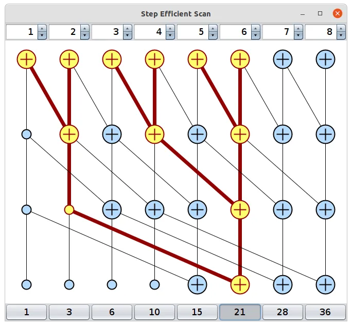
Luckily there’s an associative function we can utilize for our new activiationless RNN layers.

$f((W_1, x_1), (W_2, x_2)) = (W_1 W_2, W_1 x_1 + x_2)$

Now, we are able to apply this function do our recurrence in $O(N\log(N))$ (we are folding in $W_h$ and $W_x$ together). But, there is an additional problem where we have to store $W_i W_j \dots W_k$ during the scanning which results in a very large cubic cache as we have to store a ${\rm I\!R}^{d \times d}$ matrix for each input during the Blelloch scan. Luckily, because $W_i \in {\rm I\!R}^{d \times d}$, we can easily diagonalize these intermediate products and keep our cache quadratic.¹

Boom! Now we have a quick and parallelizable RNN. To add nonlinearity (which we still want), we can simply add an additional layer to our RNN which is applied to the recurrent part’s outputs (just like the feed forward layer after self-attention layers).

Avoiding Exploding/Vanishing Gradients

RNNs are incredibly sensitive and any small errors could result in exploding/vanishing gradients such that the our model never converges. Further, we can’t make use of gradient truncation as it would superficially make our model short range.

The solution is how we initialize our weights. If we make them very small, our gradients will be small as well. The creators of Linear RNN initialize each parameter $w$ such that

$w = e^{-e^a}e^{ib}, e^{-e^a} \sim \text{Uniform}([0.999, 1.0]), b \sim \text{Uniform}([0, \frac{\pi}{10}])$

On the other hand, our parameters are also very sensitive to inputs. We want to reduce their magnitude as much as possible. So, we multiply each input by $\Delta = \sqrt{1 - e^{-e^a}}$. From there, we’re done! ²

Mamba

Mamba improves upon using one key idea: selection. With just a recurrent network, after many iterations, it is very easy to have to hold too much information in $h_t$. The RNN should have some idea of attention — what should be retained in $h_t$ and what should be removed?

The eloquent solution, as expected, is gates. We want $W_h$ and $W_x$ (preserving notation from traditional RNNs) to be dependent on $x_i$ itself. Below shows the exact psuedocode for an SSM algorithm.³

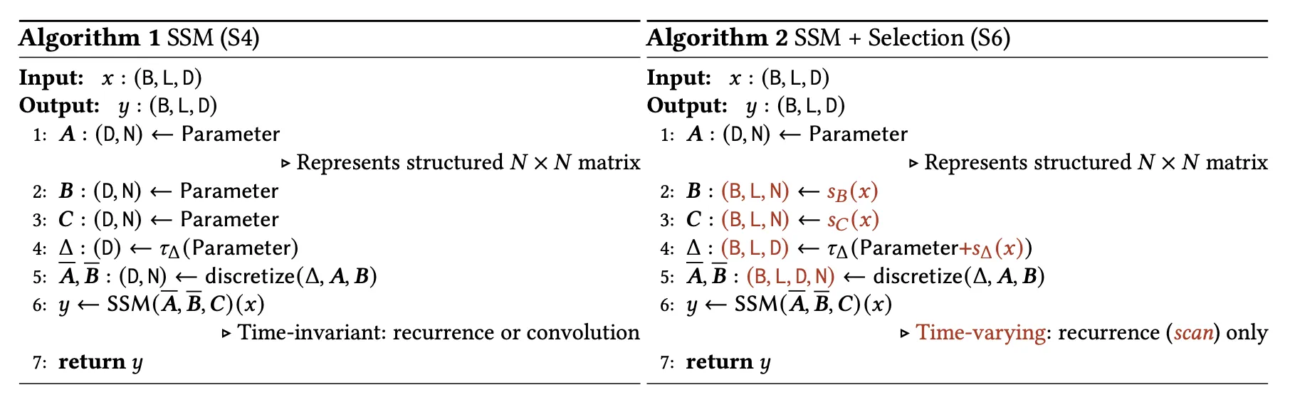
The most important thing about this algorithm is that the “selecting” functions and latent parameters⁴ (specifically $A$ and $B$) can be chosen such that $A=-1$, $B=1$, $s_\Delta = \text{Linear}(x_t)$, and $\tau_\Delta = \text{softplus}$ where the result is that each channel of our RNN having a gate is characterizable by

$\begin{aligned} g_t &= \sigma(\text{Linear}(x_t)) \\ h_t &= (1 - g_t)h_{t-1} + g_tx_t \end{aligned}$

This provides us an intuitive gate and shows us that we are really just considering how much we want to “remember” the current input at each timestep. Now, we can selectively recall information in very long context windows. Not to mention, our recurrence is only $O(N \log N)$ with the parallelization step.⁵ Now, we have Mamba!