MRI Reconstruction and Convex Optimization

This is an introduction to the MRI Reconstruction problem and approaching them with unrolled networks that I’ve been utilizing recently as a part of the MICCAI 2024 Challenge. This approach is very applicable to other impactful computer vision tasks such as image inpainting, denoising, demosaicing, etc.

Papers + Additional Resources

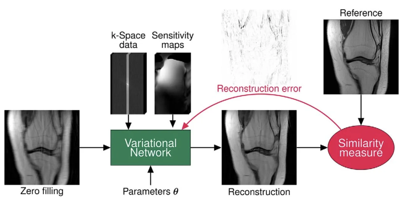
• Learning a Variational Network for Reconstruction of Accelerated MRI Data
• Nonlinear total variation based noise removal algorithms

The Problem

Say we want to take an MR image quicker. This makes the patient need to spend less time in the machine and makes physiological movement (e.g. bloodflow) less disrupting to the final image. However, in order to take an MR image quicker, we have less time to fully sample the patient’s anatomy in the scanner.

Therefore, the problem of MRI reconstruction is simple: we have an undersampled MR image and we want to reconstruct what the underlying image is. Let us define $\hat{y} = Ex$ where $x$ is our true underlying image, $\hat{y}$ is the undersampled image, and $E$ is some known function that our MRI machine is doing while taking its image defined by coil sensitivity maps, Fourier transforms, and a selected sampling pattern.

Knowing $\hat{y}$ and $E$, we want to find $x$. In other words, we hope to find $\arg\min_x {||\hat{y} - Ex||}_2^2$ to solve the ill-posed inverse problem. As with many other minimizing problems, gradient descent can solve this easily.

However, the immediate issue we see is that the image we receive from our machine is not exactly what we expect. Any machine will produce noise. Therefore, we must have a regularizer:

$\arg\min_{x} \| E x - \hat{y} \|_2^2 + \mathcal{R}(x)$

This problem is not very trivial to solve — especially if $\mathcal{R}(u)$ is not strictly known. Existing methods, such as the TV semi-norm which evaluates $\mathbf{D}$, the finite differences approximation of the image gradient, have been useful.

$\begin{aligned} \mathcal{R}(\mathbf{x}) &= \| (\mathbf{D}\mathbf{x}_{\text{re}}, \mathbf{D}\mathbf{x}_{\text{im}}) \|_{2,1} \\ &= \sum_{l=1}^{N} \sqrt{ |\mathbf{D}\mathbf{x}_{\text{re}}|_{l,1}^2 + |\mathbf{D}\mathbf{x}_{\text{im}}|_{l,1}^2 + |\mathbf{D}\mathbf{x}_{\text{re}}|_{l,2}^2 + |\mathbf{D}\mathbf{x}_{\text{im}}|_{l,2}^2 }, \end{aligned}$

However, this solution restricts the regularizer to favoring only image qualities (e.g. sparsity in image edges). Due to the complex structure of MR images, a more adaptive regularizer is necessary.

Convex Optimization with Variable Splitting

In order to converge upon this optimal $x$, we utilize variable splitting to unroll this algorithm into its two components. First, we have the Proximal Gradient step where we aim to find an image that minimizes our regularization function. Second, we have the Data Consistency step, where we propose to utilize the Conjugate Gradient method for reducing the distance between $E x$ and $\hat{y}$.

These algorithmic goals are visible through the following equations:

$\begin{aligned} u^{(i)} &= \arg\min_{u} \mu \| x^{(i-1)} - u \|_2^2 + \mathcal{R}(u) \\ x^{(i)} &= \arg\min_{x} \| E x - y \|_2^2 + \mu \| u^{(i)} - x \|_2^2 \end{aligned}$

Intuitively, if we can’t easily find a solution to the equation by utilizing gradient descent on one variable, why not split the variable $x$ into $x$ and $u$? We emphasize these variables are the “same” by the L2 distance in each minimizer, weighted by $\mu$ according to how much this is a priority.

The Proximal Gradient step

We can view the Proximal Gradient step in solving for $u^{(i)}$ as a black box modeled by a UNet, which aims to learn the correct regularization parameters by minimizing the L2 loss between the $u^{(i)}$ and the reference image. After all, the best regularizer is one that gets closest to the most optimal reconstruction. As a result, $\mu \| x^{(i-1)} - u \|_2^2$ essentially gets folded into the model and $\mu$ does not need to be explicitly defined.

The Conjugate Gradient step

Contrarily, for $\mathbf{x}^{(i)}$, we must aim to solve an inverse equation which has no machine-learnable unknowns.

In order to do solve this minimum, we can do some linear algebra with our data consistency equation:

$\begin{aligned} x^{(i)} &= \arg\min_{x} \left\| E x - y \right\|_2^2 + \mu \left\| u^{(i)} - x \right\|_2^2 \\[1ex] &= \arg\min_{x} \left[ (E x - y)^\dagger (E x - y) + \mu (u^{(i)} - x)^\dagger (u^{(i)} - x) \right] \\[2ex] &= \arg\min_{x} \left[ x^\dagger (E^\dagger E + \mu I) x - (E^\dagger y + \mu u^{(i)})^\dagger x - x^\dagger (E^\dagger y + \mu u^{(i)}) + \text{constant} \right] \\[2ex] &\Downarrow \text{Find minimizer} \\[1ex] \frac{\partial f(x)}{\partial x} &= 2 (E^\dagger E + \mu I) x - 2 (E^\dagger y + \mu u^{(i)}) = 0 \\[2ex] &\Downarrow \text{Rearranging} \\[1ex] (E^\dagger E + \mu I) x &= E^\dagger y + \mu u^{(i)} \\[2ex] &\Downarrow \text{ Solve for } x \\[1ex] x &= (E^\dagger E + \mu I)^{-1} (E^\dagger y + \mu u^{(i)}) \end{aligned}$

Luckily, $E^\dagger E + \mu I$ is characteristically a positive semi-definite matrix which allows for us to apply the Conjugate Gradient method to solve this inverse equation.

Image Reconstruction

Now that we have both parts, we just have to iterate over these steps back-and-forth to converge upon our reconstructed image! Intuitively, we are