Minimum Consistency Models pt. 1

This is an elaboration upon a talk I gave at K-Scale Labs with these slides and this GitHub repo.

Diffusion models and flow matching have been very impactful fields of recent years, and this post serves as hopefully a useful introduction. However, this will focus on more of the computer science than math, and will primarily hand-wave over a lot of the deeper theorems that require a lot more proving to reach the final goal.

Papers + Resources

Some sources to look for more insight + math:

• Flow Matching for Generative Modeling
• Consistency Models
• Diffusion Models from Scratch
• What are Diffusion Models?

The Problem

How do you get from pure noise to meaningful images in just a few iterations of a model? The motivation is simple: we want to be able to generate images similar to our training dataset not only accurately but quickly.

If you’ve heard of diffusion modeling, this may seem a bit odd. Diffusion modeling is iterating over numerous sequences of iteratively applied noise, and training a model to predict the noise that has just been added at each iteration. Inherently, this seems impossible to do in just a few steps. If we can revert from noise to meaningful images in just a few steps, this would mean we must be able to go from meaningful images to noise very quickly. However, if we were just to trivially add or subtract noise to an image — even randomize the positions of pixels in the image — we still wouldn’t get to noise in just a few steps. There needs to be a direct path.

This is where we think of Optimal Transport (OT), an optimal path between noise and a final image. This makes our earlier intuition more clear. If we think of each iterative application of our model on the a noisy image as following its learned trajectory of the path, the graph below shows how we would be less likely to converge with naive diffusion.

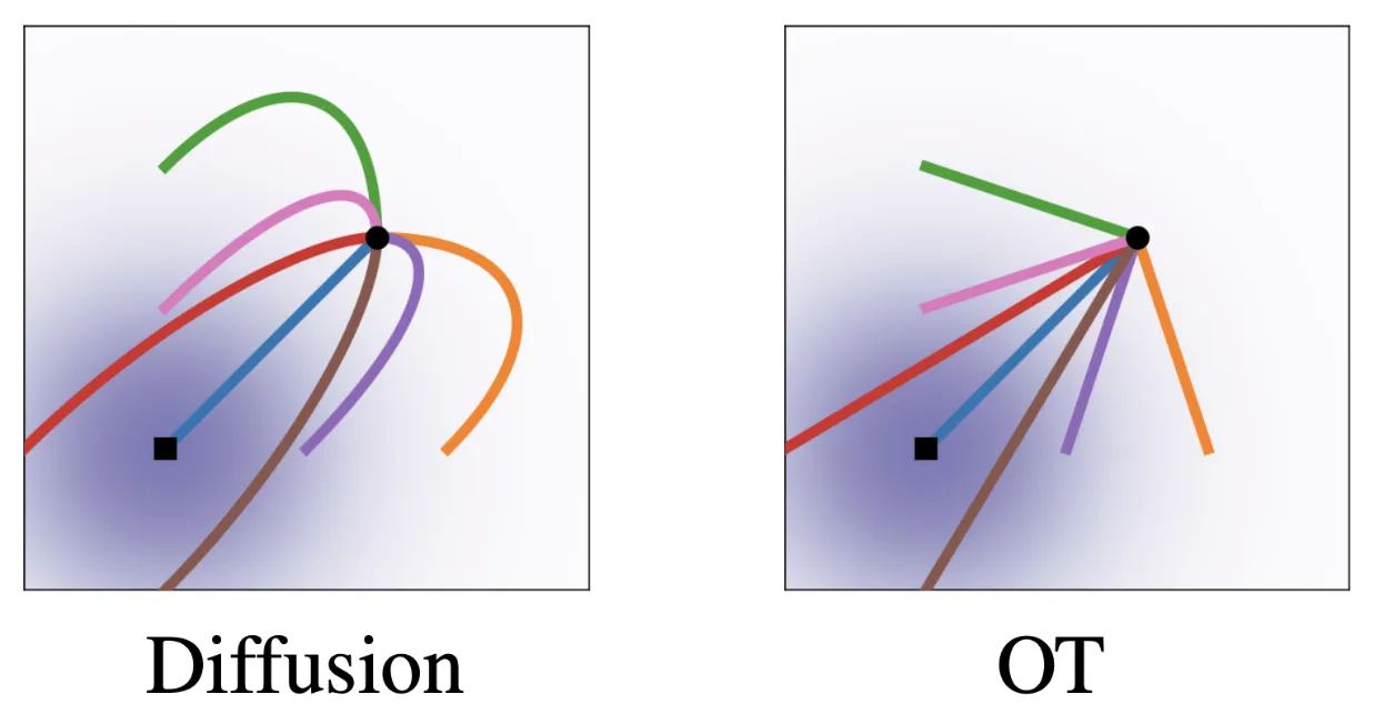
The path our model draws between noise and the ground truth image is, as expected of a random system, not direct. Thus, in a single application of the model, we would overshoot and overestimate along a dimension (unless we move very little, which is unfavorable for minimum steps possible) — the path would no longer be cleanly followed and a second iteration would act unexpectedly.

So, we agree we want the straight line. If we iterate our model once, it would move along the path and remain in a location where another iteration would still be useful. But how do we define this path?

Flow Matching

Say we have a ground truth path between noise and a true image. Surely, we want to define a function between noise and the true image. If we think of $t=0$ as where all is points generated by a Gaussian and $t=1$ as a state where all points have converged upon a ground truth image, it’s not a big stretch to say that we should define a vector field from noise to samples in our dataset.

We denote the state of our point at $t$ $\phi_t(x)$. So we can define our goal flow (the point we want x moved to after time t) as $\phi_t(x) = \sigma_t(x_1)x + \mu_t(x_1)$ where for now, $x_1$ is the only goal of our noise.

Of course, at $t=0$, $\phi_0(x)$ follows a Gaussian distribution such that $\sigma_0(x_1) = 1$ and $\mu_0(x_1) = 0$. On the contrary $\phi_1(x)$ should be centered around our ground truth image, with as minimal variance as possible. Thus, $\sigma_1(x_1) = \sigma_{min}$ and $\mu_1(x_1) = x_1$. Interpolating linearly between these values, we get $\sigma_t = 1 - (1 - \sigma_{min})t$ and $\mu_t = tx_1$.

The derivative of this flow $\phi$ defines a vector field. We want to train with this instead of the function for flow itself because this is what our model actually applies to each point as it applies changes to some initial point $x$.

So, here’s a checkpoint: in case everything above was a bit quick:¹

• We can define the path we want each point in our noise to take
• If we make it lienar, its easier to do in less steps (no overshooting or undershooting)
• Now can we learn this path?

Actual Training

Formally, we have $u_t(x|x_1)$, our ground truth vector field where we are guiding the noise towards a point over $t \in [0, 1]$

$\begin{aligned} u_t(x|x_1) & = \frac{d}{dt} \phi_t(x) \\ & = \frac{\sigma_t'(x_1)}{\sigma_t(x_1)} (x - \mu_t(x_1)) + \mu_t'(x_1) \\ \end{aligned}$

As we have defined $\sigma_t(x_1)$ and $\mu_t(x_1)$, we can substitute everything in to arrive at a final equation. The algebra is left to the reader.

Thus, we can now train a model that learns this path. First, we can generate noise and define the path we want it to take. Over many timestamps, we want it to reach a goal image from our dataset. So we train our model to learn its own vector field to turn noise into these goal images over these timestamps, minimizing the difference between predicted vector field and our pre-defined vector field.

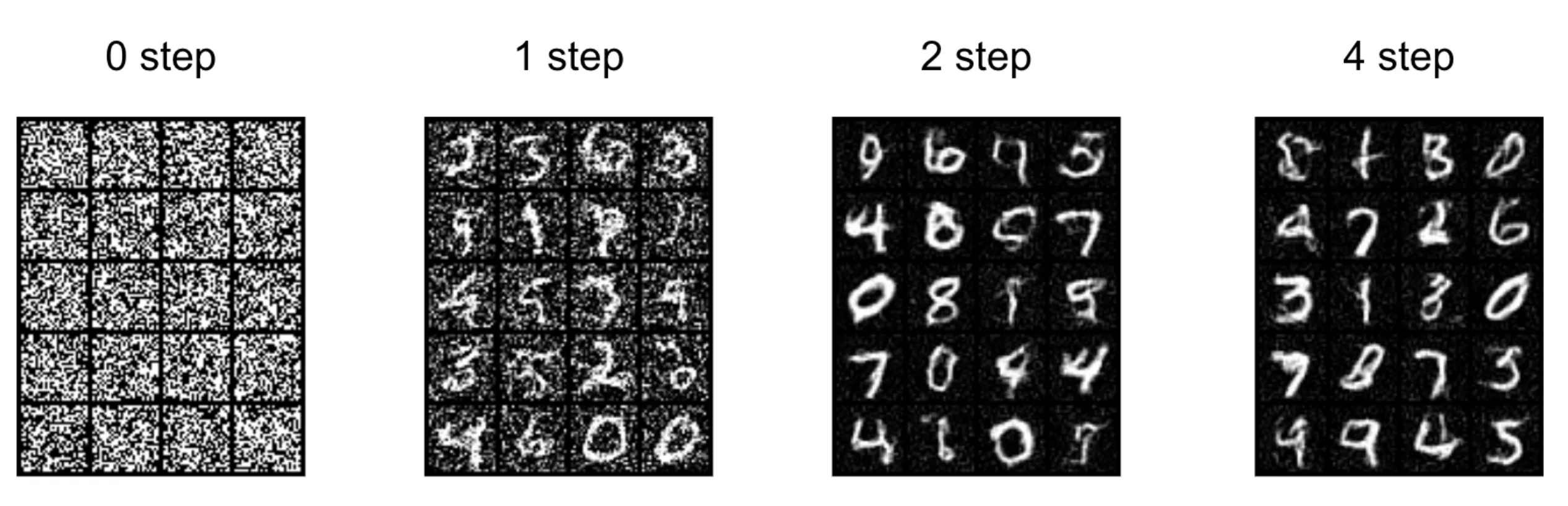
Now, we have flow matching! But spoilers: we still have to iterate our model many times in order to generate an image — too long for practical applications in speech (and too resource-intensive for large tasks like MRI image denoising). We trained using too many timestamps — even though we have a straight line path, the model makes minor progress per timestep! How can we train a model that requires less iterations as promised?

A sneak peak: